A neural texture compression and rendering experiment: an MLP is trained offline in PyTorch to compress PBR material textures into a compact latent representation, then reconstructed at runtime in a Vulkan + Slang renderer using cooperative vector / cooperative matrix acceleration. (Note: the focus of this project is reproducing the paper and exploring the neural texture compression technique, so the C++/Python code and architecture are not representative of my best engineering work.)
Neural Texture Compression
Following Random-Access Neural Compression of Material Textures, the compressor has two pieces:
- A pyramid of latent feature grids that stores per-texel features
- A small MLP decoder that decompresses those features back into PBR channels
All five PBR maps (base color, normal, AO, metal-roughness, emissive — 15 channels in total) share the same pyramid and MLP, so the network is evaluated once per shaded pixel and produces the full material vector.
Latent Pyramid
The latent storage is a pyramid indexed by mip level. Each pyramid level holds two grids:
| Grid | Resolution | Channels | Sampling |
|---|---|---|---|
G0 |
base_res / 4 (high) |
c0 = 12 |
4-nearest-neighbor concatenation |
G1 |
base_res / 8 (low) |
c1 = 20 |
bilinear |
Level 0 covers the four highest-detail mips, and each subsequent level covers two more, so the same pyramid serves the entire mip chain while keeping the high levels small.
Instead of bilinearly filtering G0 inside the trainer, its four texel neighbors are concatenated (4 × c0 = 48
features) and the MLP learns the blend itself, which preserves more high-frequency detail than a hard interpolation.
G1 is bilinearly sampled (c1 = 20 features). The final latent vector is 68 values.
Both grids are stored at 4 bits per component with asymmetric uniform quantization. During training the grids are
kept in float, perturbed with quantization noise, and clamped to the quant range every step (QAT). For the last 5% of
training the grids are hard-quantized and frozen, and only the MLP is fine-tuned. At export the grids are repacked into
VK_FORMAT_R8G8B8A8_UNORM array layers so the runtime can sample them with a regular hardware sampler.
MLP Decoder
The decoder is a 2-hidden-layer MLP. Per pixel its input is:
| Input | Width | Notes |
|---|---|---|
Latent features (G0 + G1) |
68 | sampled from the pyramid |
| Positional encoding | 12 | tiled triangular wave, 3 octaves × 2 axes × (sin, cos) |
| Normalized LOD | 1 | mip / max_mip |
The hidden width is 64, the output is 15 channels with no output activation. Hidden layers use HardGELU, the paper’s cheap inference-time GELU approximation:
The positional encoding is the paper’s tiled triangular wave: a periodic pattern that repeats every 8 texels at the
highest mip with frequencies 1, 2, 4. Triangle waves are used in place of sin/cos so the encoding maps to a handful
of ALU ops at runtime.
For runtime export the FP16 weight matrices are padded so each row is a multiple of 8 elements (16 bytes), which is what the cooperative-vector path requires for row-major matmul.
Training
Per the paper (Sec. 5.1), mip levels are sampled non-uniformly, LOD = floor(-log_4 X) with X ~ U(0,1), biasing the
budget toward higher-resolution mips, with a 5% uniform fallback. Loss is MSE against the ground-truth mip. The latent
grids and the MLP are optimized jointly with separate learning rates (Adam + cosine schedule), then the QAT freeze phase
fine-tunes only the MLP against the hard-quantized grids.
Offline Output Comparison
The model is trained offline in PyTorch. The figure below shows the per-channel output:
 (From left to right: input, latent, reconstructed, diff)
Final reconstruction PSNR (vs. original, full-res):
| PSNR | MSE | |
|---|---|---|
| Albedo | 34.78 dB | 0.000332 |
| Normal | 39.06 dB | 0.000124 |
| AO | 39.55 dB | 0.000111 |
| MetallicRoughness | 35.56 dB | 0.000278 |
| Emissive | 46.95 dB | 0.000020 |
| Overall | 37.62 dB | 0.000173 |
Runtime Inference
The trained MLP is evaluated at runtime with Vulkan and Slang. As shown below, the runtime-reconstructed textures closely match the originals.
 (Left: original textures; right: runtime reconstructed textures)
Pre-reconstructing the full texture set with a compute shader using cooperative vector takes 0.744 ms with the following PSNR (vs. original, full-res):
| PSNR | |
|---|---|
| Albedo | 35.34 dB |
| Normal | 39.54 dB |
| AO | 39.78 dB |
| MetallicRoughness | 35.87 dB |
| Emissive | 47.03 dB |
| Overall | 38.03 dB |
Full-screen Inference
Per-frame cost when reconstructing at run-time during shading:
I tested a baseline shader without acceleration, then with cooperative vector and cooperative matrix paths:
| Performance (GPU) | |
|---|---|
| Traditional Forward PBR (with reconstructed textures) | 0.103 ms |
| Neural Rendering Forward Pass (Coop Vec) | 0.402 ms |
| Neural Rendering Deferred Pass (No Acceleration) | 5.380 ms |
| Neural Rendering Deferred Pass (Coop Vec) | 0.474 ms |
| Neural Rendering Deferred Pass (Coop Mat) | 1.901 ms |
Filtering
Pre-reconstructed textures look fine, but real-time reconstruction shows visible blocky artifacts when zoomed in:
To reduce the artifacts, I applied bilinear filtering during sampling. Results below (the cooperative matrix deferred path is omitted because it is too slow to be useful here):
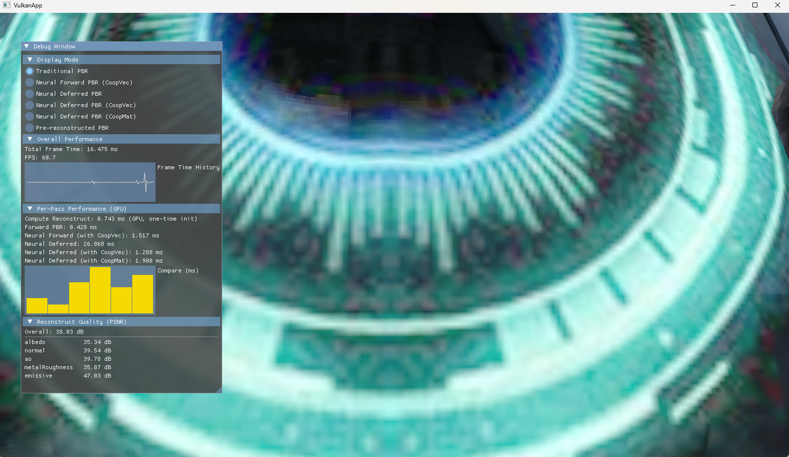
| Performance (GPU) | |
|---|---|
| Traditional Forward PBR (with original textures) | 0.428 ms |
| Neural Rendering Forward Pass (Coop Vec) | 1.517 ms |
| Neural Rendering Deferred Pass (No Acceleration) | 26.868 ms |
| Neural Rendering Deferred Pass (Coop Vec) | 1.288 ms |